

If you're working with AI applications be it recommendation systems, chatbots, RAG pipelines, or even anomaly detection you've probably crossed paths with vector search. But here’s the thing: not all vector search methods are built the same.
At its core, vector search is about retrieving information not by exact keyword match, but by meaning. Each item (text, image, code snippet) is represented as a vector in high-dimensional space. The goal? Find the “closest” ones to your query vector. But how we define “close” and how we scale that across millions (or billions) of items is where things get interesting.

In today’s edition of Where’s The Future in Tech let’s go through five key vector search methods that every developer should understand.
What Exactly Is Vector Search?
At a high level, vector search is about retrieving data based on meaning, not just keywords. In traditional search (like Elasticsearch or SQL), if I look up “healthy food,” the engine searches for documents that contain the exact words “healthy” and “food.” It doesn’t understand that "kale smoothie" might be relevant, even if those exact words never appear.
But in vector search, every item (a document, image, video, etc.) is embedded into a numerical vector a dense, high-dimensional representation that captures its meaning. Similarly, when you search for something, your query is also converted into a vector. The engine then finds which items are nearest to that query vector using math, not just words.
The underlying idea is:
Semantic similarity = vector proximity.
A Quick Example:
Imagine we have these three document embeddings:
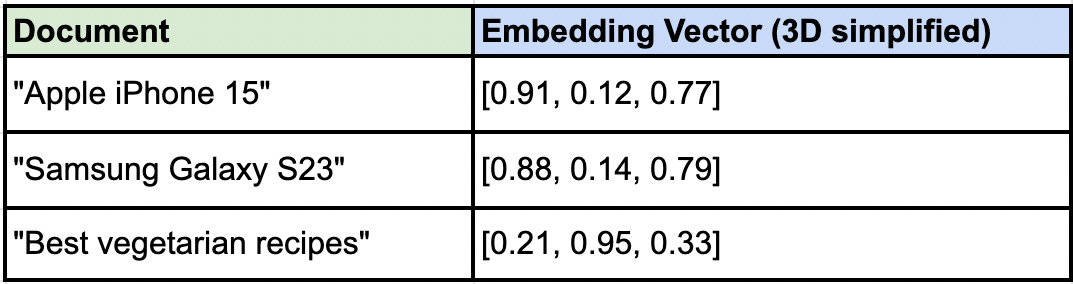
And your query vector is [0.90, 0.13, 0.76] clearly, the iPhone and Galaxy documents are much closer (in Euclidean distance or cosine similarity) to the query than the recipe doc. This is vector search in action simple idea, massive implications.
What’s a Vector Database?
Once you’re dealing with hundreds, thousands, or millions of these vectors, you need a way to store, index, and retrieve them efficiently. That’s where vector databases come in.
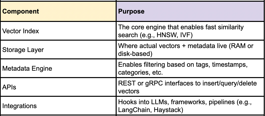
A vector database is purpose-built to handle:
Storage of high-dimensional vectors
Efficient similarity search (via Approximate Nearest Neighbor or ANN algorithms)
Metadata filtering (e.g., “only show me documents from 2023”)
Real-time updates and deletions
Integration with LLMs and multimodal pipelines
While traditional databases (like PostgreSQL or MongoDB) focus on structured or document-based data, vector databases specialize in unstructured, embedding-based data.
Anatomy of a Vector DB
Let’s Dive In: 5 Core Methods of Vector Search in Databases
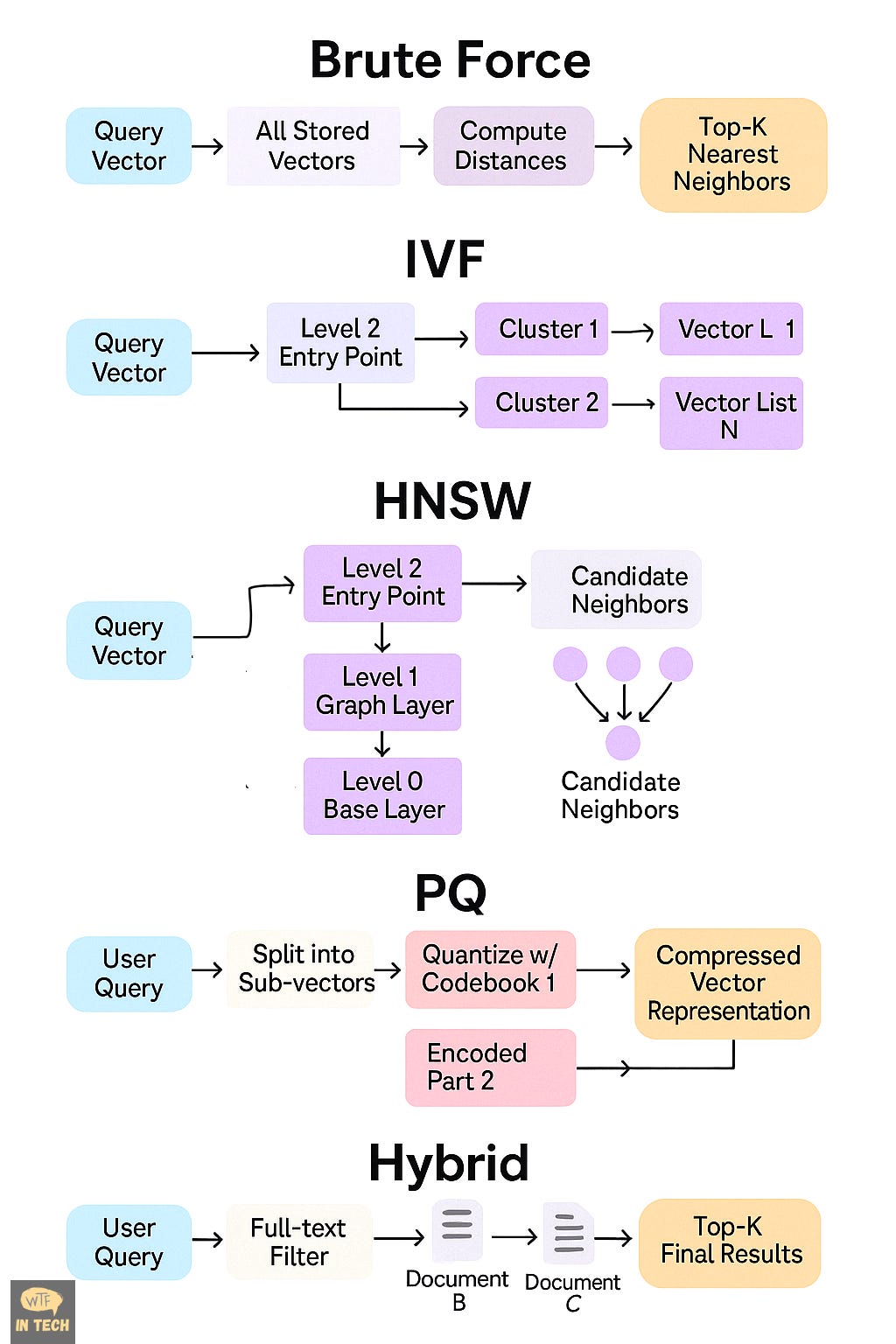
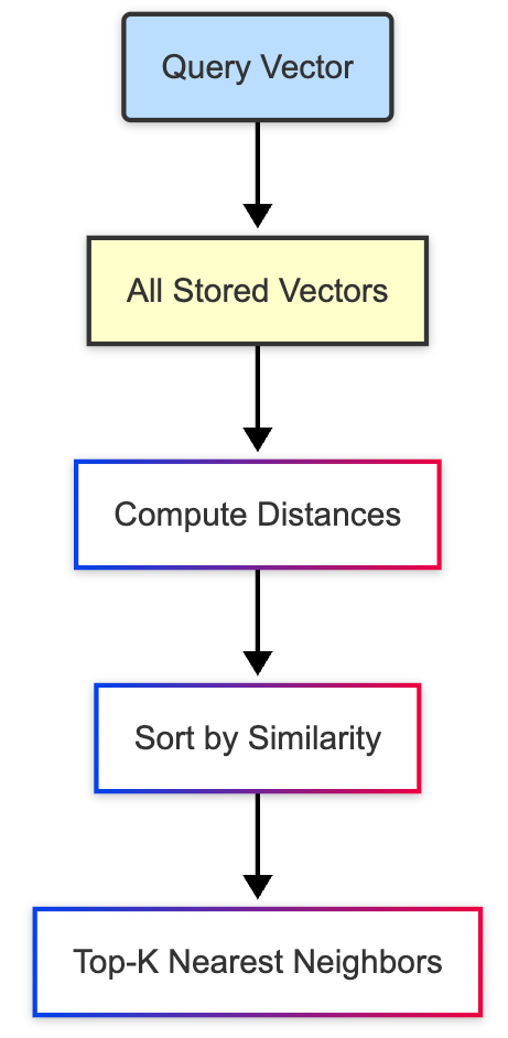
1. Brute-Force
Imagine walking into a library and comparing every single book to your query, page by page. That’s brute-force search. It doesn’t cut corners. It doesn’t guess. It just exhaustively computes the distance between your query vector and every single vector stored in the system.
Is it smart? Not particularly.
Is it effective? Absolutely for small datasets.
Is it scalable? Not in the slightest.
But once your database hits tens or hundreds of thousands of vectors, brute-force starts feeling like dialing rotary phones in the age of smartphones. It’s charming, but inefficient.
Query Vector
     ↓
[Distance Calculator] ← compares → [All Stored Vectors]
     ↓
Sorted List of Nearest Neighbors
How it works:
Query vector is compared to every vector using distance metrics.
Top-K closest results are returned.
No approximation. Pure math.
Tech underneath:
Vector math libraries like NumPy or BLAS
Often accelerated with GPUs (e.g., FAISS’s IndexFlatL2)
2. IVF: Divide and Search
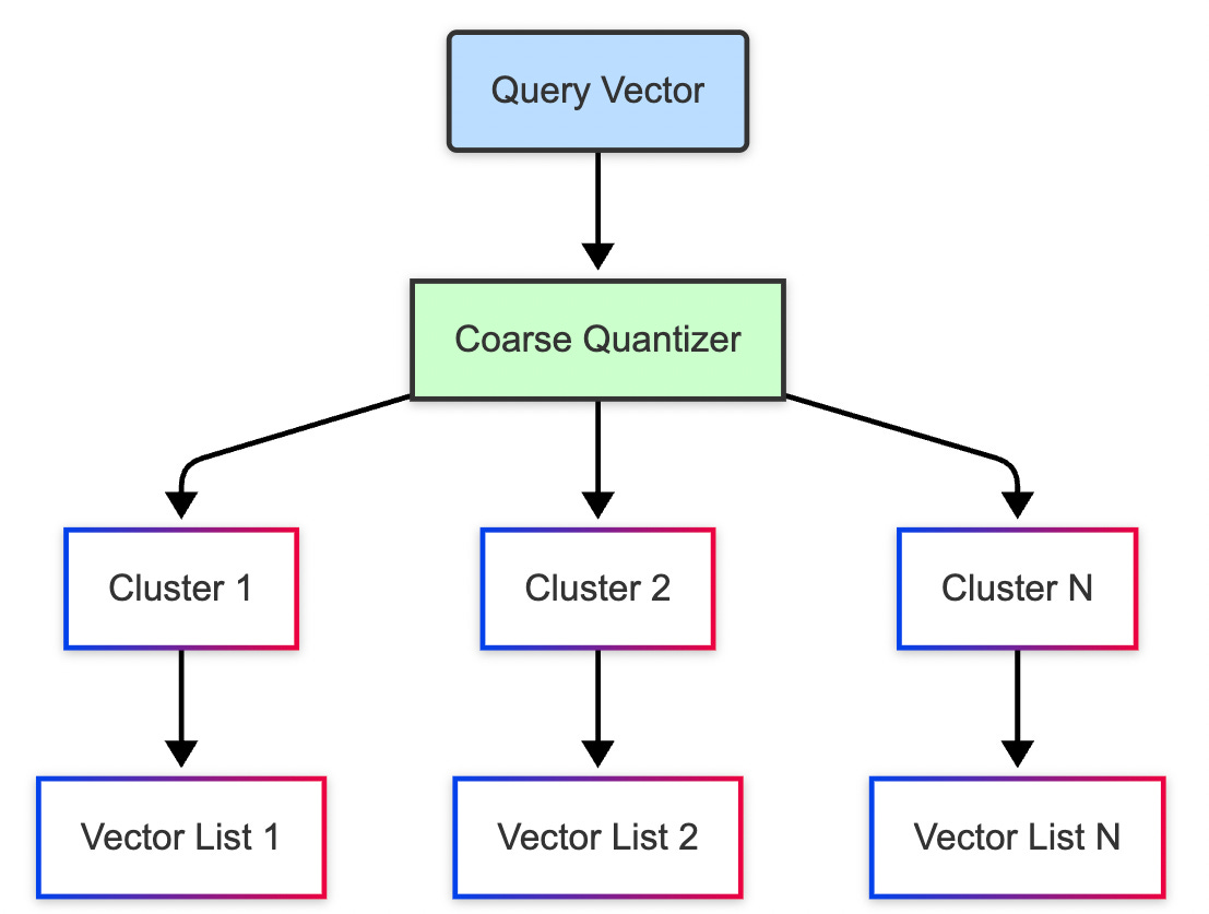
Now, say you want to be clever about it. You split the library into rooms based on topic physics, philosophy, fashion and only check the most relevant room based on what you’re looking for. This is the intuition behind Inverted File Indexing, or IVF.
Instead of treating all vectors equally, IVF first organizes them into clusters like neighborhoods on a map. Then, when a new query comes in, it doesn’t scan the whole map. It just walks into the two or three neighborhoods closest to the query and looks for answers there.
The genius lies in this compromise: you're not checking every possibility, but you're checking the most likely ones. It's faster than brute-force, and you can control how much you want to trade accuracy for speed just increase or decrease how many clusters you search.
Of course, it needs a bit of prep work upfront. Clustering takes time, and the results depend on how well those clusters are formed. But in mid-sized workloads say, under 10 million vectors IVF can hit that sweet spot between fast and fairly accurate.
[Query Vector]
     ↓
[Search in Top Graph Layer (Sparse)]
     ↓
[Zoom into Lower Layers (Denser)]
     ↓
[Find Closest Vectors]
How it works:
Indexing phase:
The vector space is divided using k-means clustering (you pick how many).
Each cluster is associated with a centroid and an inverted list.
Search phase:
Query vector is assigned to the closest centroid(s).
Search happens only inside those lists not the entire dataset.
Key parameters:
nlist: How many clusters you split intonprobe: How many clusters to search at query time
3. HNSW: Graphs, But Make It Navigable
IVF is great, but what if the vector space isn’t so cleanly divisible into neighborhoods? What if we want something more fluid like a road network that lets us drive toward our goal, even if we don’t know exactly where it is?
Enter HNSW, the name is a mouthful Hierarchical Navigable Small World but the idea is beautifully intuitive: organize your vectors into a graph where each point knows its closest friends. Then, when a query arrives, you use those friendships to “hop” your way toward the nearest match.
The result? Blazingly fast, highly accurate search. HNSW is the current gold standard for most real-time applications, especially in high-dimensional data like image embeddings or LLM-generated document vectors.
It’s not perfect. It takes time and memory to build the graph, and tuning it can be a bit like adjusting the sails of a very fast ship rewarding, but sensitive. But for production systems that need speed and scale, HNSW is often the default choice.
Step 1: Clustering Vectors → [Centroid 1, Centroid 2, ..., Centroid N]

Step 2: Store each vector in its nearest centroid’s "bucket"

Step 3: At search time → Match query to a centroid → Search only in that cluster
How it works:
Build a multi-layer graph:
Top layers have fewer nodes (coarse search)
Bottom layers are dense and accurate
Query starts at the top layer and “navigates” down the graph using greedy search
Traversal is efficient and converges toward nearest neighbors
Important terms:
M: Max neighbors per node (higher M = more edges = higher accuracy)ef: Candidate pool size during search (larger = better recall, slower speed)
4. PQ: Compression With a Purpose
Speed is great. But what if your dataset is so massive that it doesn’t even fit in RAM?
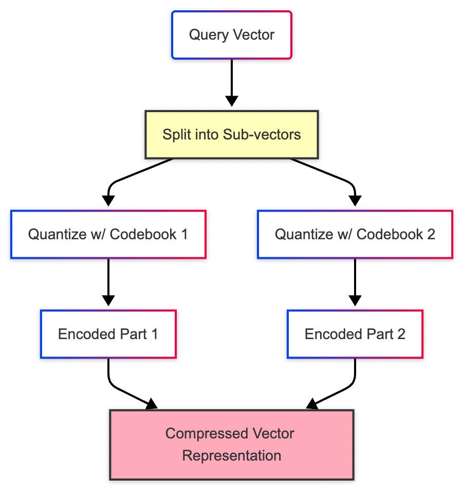
That’s when we pull out the secret weapon: Product Quantization, or PQ. This method doesn’t try to search faster it tries to store smarter. Instead of saving full precision vectors, it breaks each vector into chunks and represents each chunk with a compact code from a predefined dictionary.
It’s like writing notes in shorthand. The original meaning is mostly there, but the storage footprint is dramatically smaller.
Now, when a query comes in, it’s not compared to the original data it’s matched against these compressed codes using lookup tables. The results aren’t pixel-perfect, but they’re usually close enough. And suddenly, you can run billion-scale searches on a single machine.
Of course, you sacrifice a bit of accuracy in the process. But when you need to store and search through billions of vectors, PQ turns out to be the only way to make it all fit without breaking the bank.
[Original Vector] → [Chunked] → [Quantized] → [Stored as Codebook Entries]

[Query Vector] → [Chunked] → [Compare with Codebooks] → [Estimate Distance]
How it works:
Each vector is split into smaller sub-vectors.
Each sub-vector is quantized (mapped) to the nearest entry in a small codebook.
Instead of storing the full vector, we store only the codebook indices.
At query time, distances are computed using lookup tables super fast!
Key concepts:
Codebook: A predefined set of representative sub-vectors
Subspace decomposition: Vector = [A | B | C | D] → each part gets compressed
5. Hybrid Search: The Best of All Worlds?
By now, you might be wondering why pick just one?
Good question. And modern vector systems are asking the same thing. Increasingly, we see hybrid architectures that blend these methods together:
IVF for coarse filtering
HNSW for refined navigation
PQ for memory efficiency
This hybrid approach allows systems to balance latency, memory, and accuracy like a pro DJ balancing bass and treble. Tools like FAISS, Qdrant, Weaviate, and Milvus often expose multiple strategies that can be stacked or toggled depending on the use case.
In essence, there’s no one-size-fits-all. The method you choose depends on your data size, your latency budget, your memory limits, and your accuracy demands. The real art lies in knowing which lever to pull.
Step 1: Approx Search (IVF/PQ/HNSW)

Step 2: Get Top-N Candidates

Step 3: Brute-Force Re-Ranking of Top-N

Step 4: Final Sorted Top-K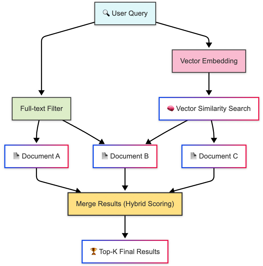
Here’s how it flows:
Filter first: Narrow down the data using classic filters (e.g., category = “laptops”, date > last 30 days).
Fast vector search: Use an ANN method like HNSW or IVF to find vectors semantically close to the query.
Smart rerank: Blend in other factors like ratings, recency, or use a reranking model to fine-tune the top results.
Final Thoughts
At the end of the day, vector search isn't just about finding the "nearest neighbor" it's about balancing accuracy, speed, and scale based on your real-world needs.
Need lightning-fast results for millions of vectors? HNSW or IVF might be your heroes. Working in a memory-tight environment? PQ’s your best friend. Want total precision no matter the cost? Brute force will never lie to you. And if you're like me forever torn between performance and perfection hybrid methods with re-ranking often hit that sweet spot.
Just like choosing the right database engine or API architecture, picking a vector search method is a design decision. One that should evolve with your product’s scale, traffic, and intelligence layer.
So next time you're building that search system, chatbot retriever, or personalized recommender pause for a second. Ask: "Am I using the right kind of vector?" Because in the future of tech, how you search is just as important as what you find.

Until next time,
Stay curious, stay innovative and subscribe to us to get more such informative newsletters.